Indicators
Tuesday, June 9th 2020
Describing The Implied Volatility Options Surface
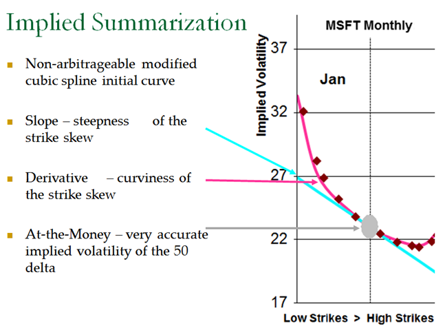
ORATS summarizes the implied volatility skew into slope, derivative, and fixed day points after drawing a smooth curve through the strike IVs.
Summary
ORATS describes the implied volatility surface as a 3-dimensional surface where the independent variables are time to expiration, and option delta and the dependent variable is implied volatility. ORATS measures the surface using at-the-money volatility, strike slope, and derivative (curvature) to give traders a macro view of the implied volatilities for each option chain. ORATS takes a snapshot of all options on all symbols approximately 14 minutes before the close of trading. The slope and derivative are used to create parameters for comparison to other months in the same security and to other securities.
ORATS describes the implied volatility surface as a 3-dimensional surface where the independent variables are time to expiration, and option delta and the dependent variable is implied volatility. To illustrate an implied volatility surface, we have developed a 2-dimensional graph that displays all three axes in the figure below. Summary information about this surface gives the trader a macro view of the implied volatilities for each option chain. ORATS takes a snapshot of all options on all symbols approximately 14 minutes before the close of trading. Options markets from this time are often of higher quality than at the close.
ORATS measures the surface using the following summary characteristics: at-the-money volatility, strike slope, and derivative (curvature).
Delta is best to use on the x-axis as was said earlier it normalizes the skew so you can compare different expirations and different stocks.
Strike Slope is a measure of the amount that implied volatility changes for every increase of 10 call delta points within the intra-month skew. It measures how lopsided the 'smile' or 'smirk' is. The derivative is a measure of the rate at which the strike slope changes for every increase of 10 call delta points within the intra-month skew. It measures the curvature of the intra-month skew or 'smile.' We chose just two parameters to describe the skew to get a reasonable fit for the fewest assumptions.
We start with lining up the calls and puts IVs using residual yields. We use the 85 to 15 call deltas in the study. We have more weightings to the call an puts for closeness to the 50 delta and we weight the call vs put the more OTM we go, meaning the 20 delta call IV will get more weighting than the same strike 80 delta put: The IVs will be slightly different even after our residual yield process. Then on to estimating the slope with a best fit, and we are left with errors from the slope line to the actual mid market IVs. We apply the derivative to minimize those errors.
We create a slope & derivative not to create our smooth market values but to create parameters for comparison to other months in the same security and to other securities.Our smooth market values process starts with a process akin to a cubic spline and then this spline is adjusted to strike IVs in a localized methodology. This process creates a very accurate theoretical values to the market bid-ask, being in between ~99% of the time.After the SMV process we then calculate a slope & derivative. This is an intricate process developed over many years and with much trial and error.
In our service all this can be graphed historically on our web tool or downloaded in our API.
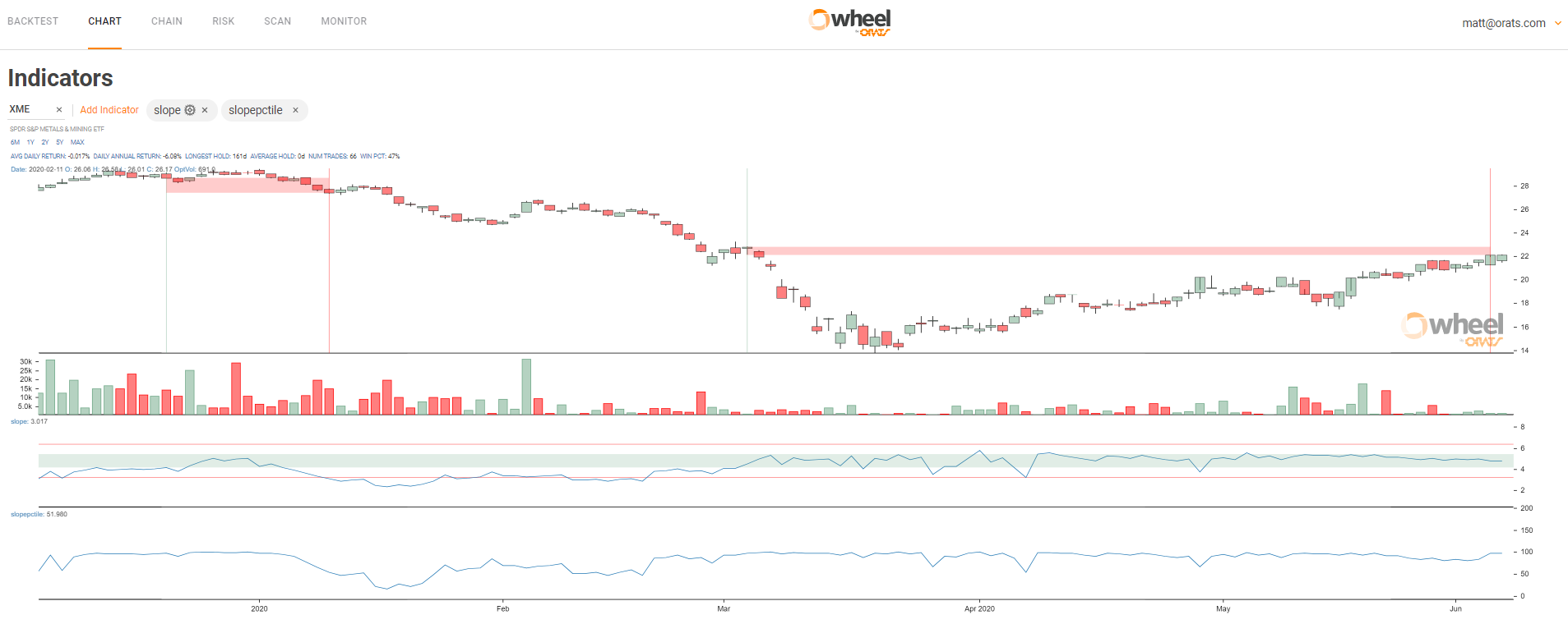
For example, IYR's slope looks cheap and XME's slope looks expensive from a variety of measurements:
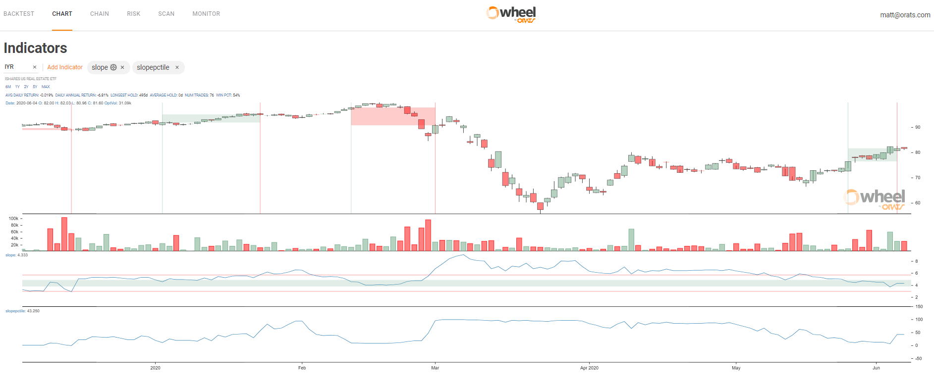
1. We have a forecast of slope and that forecast is above IYRs current slope.
2. IYR has a relatively low slope percentile vs say XME whose slope percentile is higher, see below.
3. ORATS also has a measurement of the component averages for all readings including slope, and slope percentile. The ratio of IYR's components slope to IYR's slope makes the ETF look cheap and opposite for XME.
4. We also compare the ETFs to the SPY and track the relationship. For stocks, we track the relationship of the best ETF.
If you look in our documentation you can see the names and descriptions. We also have blogs about slope.
Here are a sampling of more fields:
Notes: We use a binomial tree approach as described in Haug "The Complete Guide to Option Pricing Formulas". We use percentage of a day starting at 95% at the open and 5% at the close. Pricing models generally don't work with 0 DTE. We calculate a confidence level for each expiration, so that would be the error term for the IV. We calculate historical goodness of fit for our forecasts, and that is the error term for your comparison.
Disclaimer:
The opinions and ideas presented herein are for informational and educational purposes only and should not be construed to represent trading or investment advice tailored to your investment objectives. You should not rely solely on any content herein and we strongly encourage you to discuss any trades or investments with your broker or investment adviser, prior to execution. None of the information contained herein constitutes a recommendation that any particular security, portfolio, transaction, or investment strategy is suitable for any specific person. Option trading and investing involves risk and is not suitable for all investors.
All opinions are based upon information and systems considered reliable, but we do not warrant the completeness or accuracy, and such information should not be relied upon as such. We are under no obligation to update or correct any information herein. All statements and opinions are subject to change without notice.
Past performance is not indicative of future results. We do not, will not and cannot guarantee any specific outcome or profit. All traders and investors must be aware of the real risk of loss in following any strategy or investment discussed herein.
Owners, employees, directors, shareholders, officers, agents or representatives of ORATS may have interests or positions in securities of any company profiled herein. Specifically, such individuals or entities may buy or sell positions, and may or may not follow the information provided herein. Some or all of the positions may have been acquired prior to the publication of such information, and such positions may increase or decrease at any time. Any opinions expressed and/or information are statements of judgment as of the date of publication only.
Day trading, short term trading, options trading, and futures trading are extremely risky undertakings. They generally are not appropriate for someone with limited capital, little or no trading experience, and/ or a low tolerance for risk. Never execute a trade unless you can afford to and are prepared to lose your entire investment. In addition, certain trades may result in a loss greater than your entire investment. Always perform your own due diligence and, as appropriate, make informed decisions with the help of a licensed financial professional.
Commissions, fees and other costs associated with investing or trading may vary from broker to broker. All investors and traders are advised to speak with their stock broker or investment adviser about these costs. Be aware that certain trades that may be profitable for some may not be profitable for others, after taking into account these costs. In certain markets, investors and traders may not always be able to buy or sell a position at the price discussed, and consequently not be able to take advantage of certain trades discussed herein.
Be sure to read the OCCs Characteristics and Risks of Standardized Options to learn more about options trading.
Related Posts