Indicators
Monday, June 29th 2020
Forecasting The Options Volatility Surface
Forecasting the implied volatility surface requires observations of statistical volatility, slope, derivative and earnings effects and can help assess market prices of options.
Summary
Forecasting the options volatility surface requires observations of statistical volatility, slope, derivative, and earnings effects. ORATS breaks the volatility surface into several parameters, including a 20-day forecast of future statistical volatility, infinite forecast of implied volatility, earnings forecast, strike slope forecast, and curvature or derivative forecast. These observations are used in volatility forecasting models to compare implied volatility surface parameters and market values to forecasted parameters and theoretical values computed using these parameters. ORATS also produces metrics on the accuracy of these forecasts.
Making a forecast for each option can provide a guide on what to trade: What is overvalued and what is undervalued.
Before creating forecast, historical observations of skew parameters should be produced. ORATS has chosen to break the volatility surface into the following parameters:
- 20 business day (~1 month calendar) forecast of future statistical volatility - orFcst20d. This forecast is based on observations often back to 2007 of historical volatility using a modified Parkinson method.
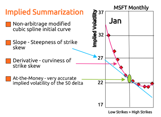
- Infinite forecast of implied volatility - orFcstInf. This forecast is based on observations of summarized implied volatility.
- Earnings forecast - fcstErnEffct. ORATS forecasted earnings effect considers day of and day after earnings, seasonality, recentness, median and average of move divided by expected move.
- Strike slope forecast and infinite slope forecast, slopeFcst, slopeFcstInf. Observations of slope forecasted.
- Curvature or derivative forecast - derivFcst, derivFcstInf. Observations of derivative forecasted.
These sophisticated methods of summarizing and manipulating the implied volatility surface allow us to compare summary characteristics across related equities and over time. These observations are then used in volatility forecasting models. In options trading, to find an edge, it is useful to compare implied volatility surface parameters and market values to forecasted parameters and to theoretical values computed using these parameters.
We produce metrics on the accuracy of these forecasts:
- fcstR2 – is the R2 for our statistical forecast orFcst20d
- fcstR2Imp is for implied forecast orIvFcst20d
- impliedR2 is R2 for the market’s IV prediction of future HV.
Advanced: Calculating an Implied Volatility for Each Strike
Given the at-the-money implied volatility, the slope and the derivative, an implied volatility can be calculated for each strike. First, a call delta is calculated for the strike using a standard option pricing model (not provided). Second, the slope and derivative for the expiration is calculated given the interpolated slope and derivative for that expiration. Third, the implied volatility formula is used to determine the strike implied.
Formula: Atmiv*(1+(slope/1000+(deriv/1000*(delta*100-50)/2))*(delta*100-50))
For example, assume the following:
- atmIvM1: 30
- slope: 1
- deriv: 0.1
- delta: 0.75
- dte: 30
Since we are finding the month 1 volatility the 30 day slope and derivative can be used. 30*(1+(1/1000+(0.1/1000*(0.75*100-50)/2))*(0.75*100-50)) = 31.688
Example 2, assume:
- 30dayatmiv: 32
- infiniteATMIV: 28
- slope: 1
- deriv: 0.08
- slopeInf: 2
- derivInf: 0.1
- delta: 0.25
- dte: 90
In this example we first need to interpolate the IV, slope and derivative between the 30 day and in the infinite. This is done by weighting the 30day * 81% and the infinite 19% (see below).
IV = 0.81 * 32 + 0.19 * 28 = 31.26
Slope = 0.81 * 1 + 0.19 * 2 = 1.19
Derivative = 0.81 * 0.1 + 0.19 * 0.08 = 0.084
Implied volatility at 25 delta:
31.26*(1+(1.19/1000+(0.084/1000*(0.25*100-50)/2))*(0.25*100-50))=31.15
Disclaimer:
The opinions and ideas presented herein are for informational and educational purposes only and should not be construed to represent trading or investment advice tailored to your investment objectives. You should not rely solely on any content herein and we strongly encourage you to discuss any trades or investments with your broker or investment adviser, prior to execution. None of the information contained herein constitutes a recommendation that any particular security, portfolio, transaction, or investment strategy is suitable for any specific person. Option trading and investing involves risk and is not suitable for all investors.
All opinions are based upon information and systems considered reliable, but we do not warrant the completeness or accuracy, and such information should not be relied upon as such. We are under no obligation to update or correct any information herein. All statements and opinions are subject to change without notice.
Past performance is not indicative of future results. We do not, will not and cannot guarantee any specific outcome or profit. All traders and investors must be aware of the real risk of loss in following any strategy or investment discussed herein.
Owners, employees, directors, shareholders, officers, agents or representatives of ORATS may have interests or positions in securities of any company profiled herein. Specifically, such individuals or entities may buy or sell positions, and may or may not follow the information provided herein. Some or all of the positions may have been acquired prior to the publication of such information, and such positions may increase or decrease at any time. Any opinions expressed and/or information are statements of judgment as of the date of publication only.
Day trading, short term trading, options trading, and futures trading are extremely risky undertakings. They generally are not appropriate for someone with limited capital, little or no trading experience, and/ or a low tolerance for risk. Never execute a trade unless you can afford to and are prepared to lose your entire investment. In addition, certain trades may result in a loss greater than your entire investment. Always perform your own due diligence and, as appropriate, make informed decisions with the help of a licensed financial professional.
Commissions, fees and other costs associated with investing or trading may vary from broker to broker. All investors and traders are advised to speak with their stock broker or investment adviser about these costs. Be aware that certain trades that may be profitable for some may not be profitable for others, after taking into account these costs. In certain markets, investors and traders may not always be able to buy or sell a position at the price discussed, and consequently not be able to take advantage of certain trades discussed herein.
Be sure to read the OCCs Characteristics and Risks of Standardized Options to learn more about options trading.
Related Posts